

What started as a small experiment with a handful of audio recordings eventually became a system capable of processing a substantial historical backlog and then running as a daily cronjob for newly available calls. Somewhere between those two scales, the problem stopped being mainly about finding the right AI models and became a systems engineering problem.
The original question was relatively simple: could voice be used to detect when the same person called multiple times while presenting themselves under different identities? Traditional identifiers could change between calls, but the speaker's voice provided another signal. The first proof of concept only needed to demonstrate that the idea was technically viable on a small collection of recordings.
It worked.
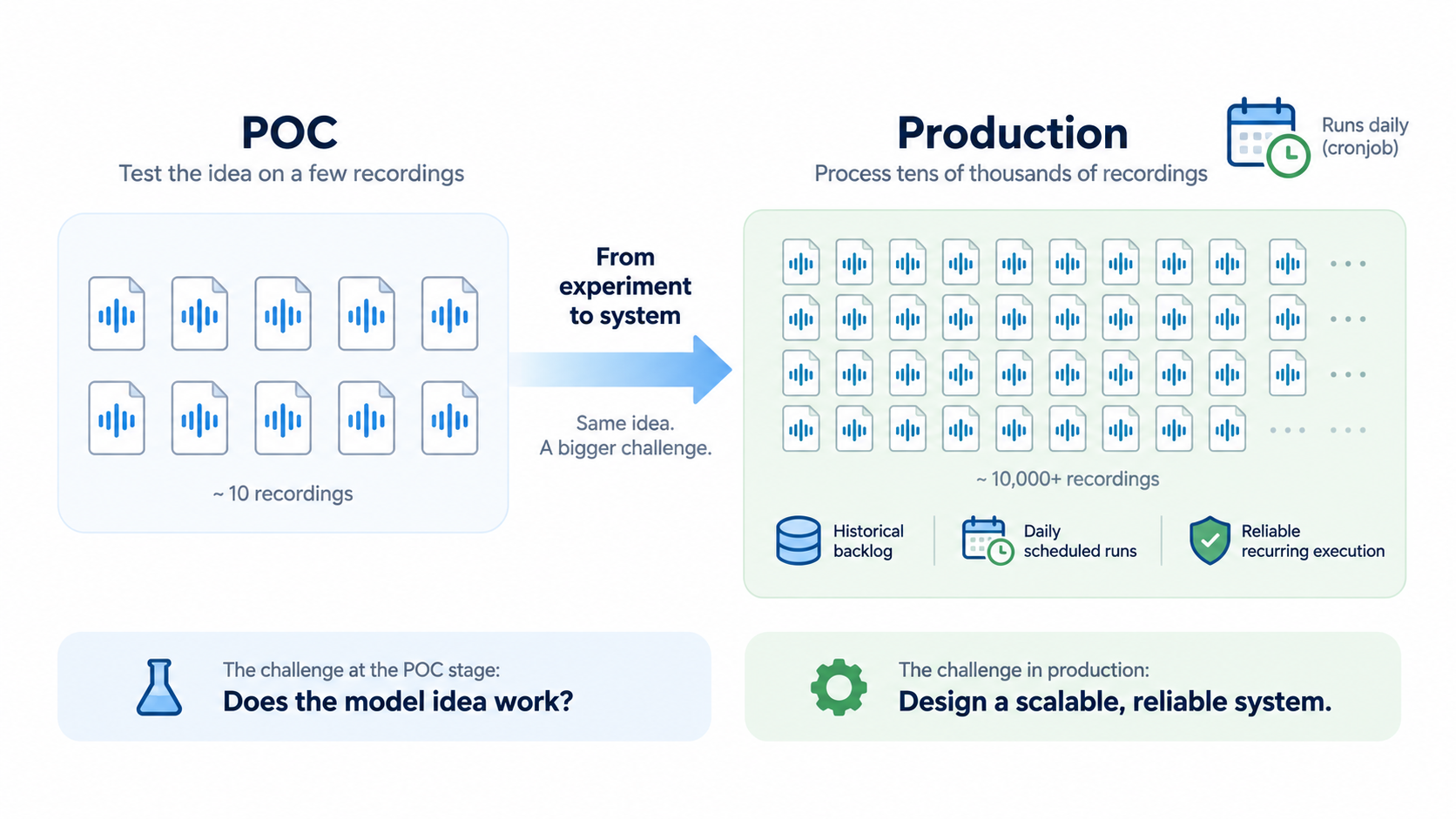
But a pipeline that works on ten recordings and one that can reliably work through tens of thousands are two very different pieces of software. As the scope expanded to include a large historical backfill followed by a daily scheduled process for newly available calls, most of the interesting engineering work shifted from proving the ML concept to designing, optimizing and operating the system around it.
Turning raw calls into the right voice
The first issue I faced was that the recordings were not clean speaker-verification samples. They were mono calls containing both sides of the conversation, with background noise, variable audio quality and speech primarily in Darija. Before I could compare voices, I had to turn those raw calls into the specific speaker audio that actually mattered.
There was also an important infrastructure constraint from the beginning: I did not have the luxury of relying on cloud services. Everything had to run locally, including audio processing, model inference, storage and vector search. That made resource management much more important. I had to work within the available CPU, GPU, memory and local storage rather than simply scaling out by sending workloads to external managed services.
The mono format immediately ruled out simply embedding the entire recording. Doing so would mix characteristics from the customer and the agent, and agents naturally occur across many different calls. Before comparing voices, I first needed to reliably extract the voice I actually wanted to compare.
I used a speaker-diarization component to split each recording into speaker-labelled segments. Diarization, however, only tells me that speaker A and speaker B exist. It does not tell me which one is the customer.
I therefore combined the acoustic result with information from the conversation itself. Agents tend to use relatively predictable greeting patterns, so I transcribed the relevant segments with a speech-recognition model and used those patterns to identify the agent. Once that attribution was made, I could discard the agent side and reconstruct customer-only audio.
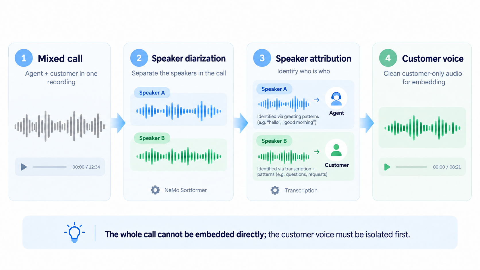
This became an important design principle throughout the project: rather than asking one model to solve an ambiguous end-to-end problem, I decomposed it into smaller problems where different signals could compensate for each other's limitations.
Finding a diarization model that worked in Darija
Diarization looked straightforward on paper, but it quickly became one of the most frustrating parts of the project.
Many diarization models perform reasonably well on clean, well-recorded speech in widely represented languages. These calls were different. They contained interruptions, overlapping speech, background noise, inconsistent recording quality and mostly Darija. A model could look impressive on a general benchmark and still produce unstable speaker boundaries or incorrect speaker assignments on this data.
I went through several models and configurations, comparing their behaviour on real recordings rather than relying only on published results. Some produced too many short segments. Others merged speakers during interruptions or split one speaker into several identities. Some were particularly sensitive to noise or silence. A few were accurate enough on individual examples but too slow or too resource-intensive for the historical backlog.
The difficulty was not simply deciding which model had the highest apparent accuracy. I also had to consider whether its output was stable enough for the downstream stages, whether it could run within the local hardware constraints, and whether its errors would make customer extraction unreliable.
This made benchmarking more complicated than comparing a single score. I had to inspect segment boundaries, speaker consistency, customer-versus-agent attribution and the quality of the resulting audio. A diarization model could produce plausible-looking labels while still creating unusable customer segments.
After testing multiple alternatives, I eventually found a diarization model that provided a much better balance for this particular setting. It was not perfect, but it was reliable enough on the Darija-heavy calls, robust enough across varying audio quality and practical enough to run as part of the full pipeline. Finding it took considerably more experimentation than the initial architecture suggested, but it made the rest of the system much more dependable.
Not every transcription model was suitable either
Transcription introduced a similar challenge.
The purpose of transcription was not to produce polished text for users. I mainly needed enough reliable text to recognize agent greeting patterns and support speaker attribution. That meant a model could be acceptable for general transcription but still fail at the specific phrases and pronunciation patterns present in these calls.
I tested several speech-recognition models and configurations. Some were too large for the available hardware and slowed down the pipeline considerably. Others handled standard Arabic or multilingual speech reasonably well but struggled with Darija, code-switching, noise or telephone-quality audio. Some produced text that looked plausible while missing the exact greeting cues needed to identify the agent.
After benchmarking the available options on representative calls, I ended up using a lightweight fine-tuned transcription model. It provided the right balance of Darija performance, speed and resource usage for the task.
These two model-selection exercises changed how I thought about benchmarking. The best model in the abstract was not necessarily the best model for the system. I needed models that worked on the actual language, audio conditions and operational constraints of the project.
Not every embedding deserves to be trusted
There was another problem hidden behind the apparently simple pipeline: a model will happily generate an embedding from bad audio.
A diarization error, a tiny speech segment, excessive silence, clipping or very poor recording quality could still produce a perfectly valid 256-dimensional vector. Syntactically valid, however, does not mean meaningful.
I introduced a quality gate using an audio-quality model together with simpler signal-level checks such as usable duration, silence and clipping. Low-quality inputs could then be rejected or treated differently rather than silently contaminating the speaker index.
For the actual speaker representation, I used a voice-embedding model to generate 256-dimensional embeddings. I stored those vectors and their associated metadata in a vector database, allowing each newly processed customer to be compared with the historical population using cosine similarity.
At this point, the ML architecture was conceptually straightforward:
raw call → diarization → speaker attribution → quality checks → customer voice → speaker embedding → vector search.
Getting that sequence to work on a few recordings was the easy part.
The point where the problem changed
The initial POC involved only a small number of recordings. Once the system had to work through a large historical backlog and then run daily as a scheduled cronjob for newly available calls, I had a different problem.
There was network ingestion, object storage, audio decoding, CPU preprocessing, multiple inference stages, GPU memory, temporary files, vector writes, similarity queries and reporting. Some operations were compute-bound. Others were I/O-bound. Some benefited from batching. Others benefited from threads. Some models needed the GPU, while other work could happen concurrently without touching it.
Because everything had to run locally, these resources were finite and shared. All of it ultimately had to work within a single high-end GPU and the surrounding local infrastructure.
Simply making each model fast was no longer enough. I needed to make the pipeline fast.
Optimizing the whole pipeline, not just GPU inference
I started by profiling where time was actually being spent rather than assuming the neural networks were automatically the bottleneck.
I separated the pipeline conceptually into I/O, CPU preparation, GPU inference, vector-database operations and post-processing. That made it possible to optimize each according to its actual workload instead of applying concurrency indiscriminately.
File transfers and object-storage reads and writes are predominantly I/O-bound, so I could use small thread pools to overlap them. While one operation was waiting on the network or storage, another could make progress. Upcoming audio could also be fetched and prepared while the GPU was still processing the current batch.
GPU work required a different strategy. More parallelism does not automatically mean more throughput on an accelerator. Too little work leaves expensive compute idle; too much creates memory pressure, additional transfers and contention. I experimented with controlled batching and concurrency to keep the GPU fed without turning GPU memory into another bottleneck.
One lesson was especially easy to miss when looking only at monitoring dashboards: 99% GPU utilization does not necessarily mean the GPU is delivering 99% of the performance it could deliver. A utilization metric generally indicates that the device has work scheduled or is not idle; it does not tell me whether the kernels are efficient, whether the workload is compute-bound, whether memory bandwidth is saturated, or whether the GPU is spending time on small, inefficient operations. A GPU can appear fully utilized while still achieving poor throughput because of kernel launch overhead, memory stalls, synchronization, data-transfer bottlenecks or suboptimal batch sizes.
That meant I had to measure more than utilization. I also looked at throughput, latency, batch size, memory usage, data-transfer time and the amount of useful work completed per unit of time. The goal was not to make a dashboard show 99%. The goal was to process more audio reliably with the available hardware.
Model lifecycle mattered too. Loading a large speech model repeatedly inside a file-processing loop is enormously wasteful at scale. Models were loaded once and reused across batches, and I avoided keeping unnecessary large models resident simultaneously when they competed for GPU memory.
This created a pipeline where work could overlap:
while the GPU processed one batch, the system could read upcoming files, prepare CPU-side inputs, write completed artifacts, or perform database operations from previous work.
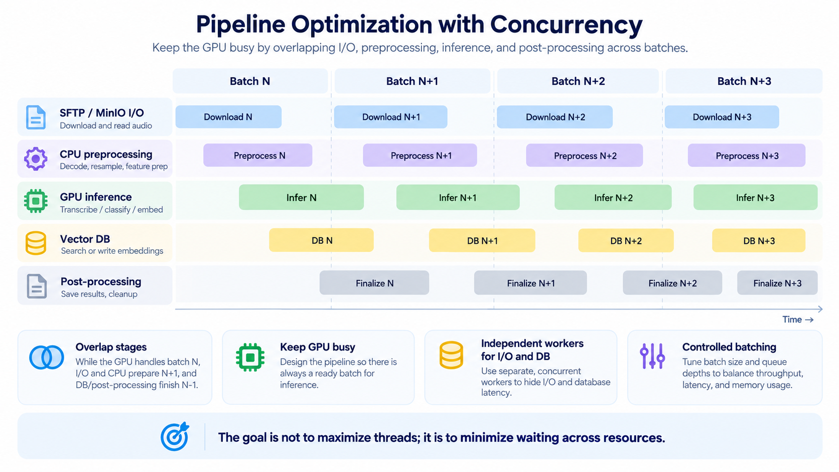
The goal was not to maximize the number of threads. It was to minimize the amount of time expensive resources spent waiting for one another.
That distinction became one of the most useful lessons from the project. Concurrency is something to optimize, not maximize, and utilization is a signal to investigate, not a performance target by itself.
Storage and database operations matter too
At this scale, seemingly small operations repeated across a large backlog become significant.
Raw recordings and intermediate artifacts were persisted in object storage rather than tied to temporary local state. I separated storage concurrency from GPU concurrency so slow object-storage operations did not unnecessarily block inference.
The same principle applied to the vector database. Issuing similarity searches or writes sequentially for every individual call creates avoidable overhead, so vector operations were batched where appropriate and searches parallelized independently from the expensive audio-processing stages.
The vector index itself was not particularly large. A collection of tens of thousands of 256-dimensional vectors is tiny compared with the underlying audio. The interesting scaling challenge was therefore not nearest-neighbour search; it was efficiently turning a large amount of messy audio into reliable vectors in the first place.
That distinction influenced where I spent optimization effort. I did not optimize the component that sounded most sophisticated. I optimized the components that profiling showed were costing the system time.
Designing for the second run, not just the first
A pipeline that takes substantial time to execute also has to assume that something will eventually fail.
A network request can time out. An audio file can be corrupted. A model invocation can fail. A process can be interrupted. If the system has already processed a significant portion of the backlog, restarting from the beginning is both slow and unnecessarily expensive.
I therefore made the pipeline idempotent.
Processing stages kept track of completed work and skipped artifacts that already existed. Intermediate results were persisted rather than living exclusively in process memory. Operations that could safely be retried were retried. Temporary files were cleaned automatically, and deterministic identifiers helped prevent duplicate vectors and duplicate processing.
The same design also mattered for daily execution. Rather than treating every cron-triggered run as a full replay, the job could identify newly available work, process it, and leave previously completed artifacts untouched. Each run therefore behaved more like an incremental update than a repeated backfill.
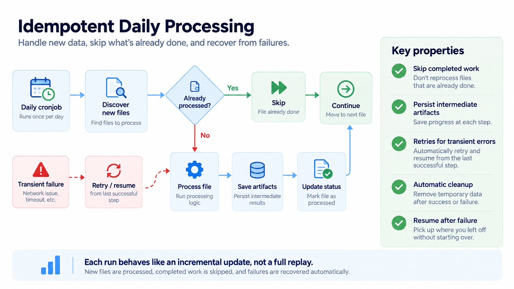
The result was that a failed run could resume from useful state instead of replaying the entire pipeline, while routine daily runs could focus on what had changed since the previous execution.
This sounds less exciting than speaker embeddings or GPU inference, but it is one of the differences between an AI demo and an AI system.
High precision was a product decision, not just a threshold
The final similarity search also required a decision about what the system should actually claim.
I deliberately used conservative similarity thresholds, with approximately 0.98 representing strong matches and around 0.95 serving as a lower candidate boundary. The system was not designed to autonomously declare that two identities belonged to the same fraudulent person. It was designed to surface high-confidence relationships for investigation.
That distinction mattered because false positives were expensive.
If this had been a recommendation system, accepting some irrelevant matches might have been harmless. Here, a false match could incorrectly associate two different people with suspicious behaviour. Lowering the similarity threshold would immediately produce more detections, but a larger number on a dashboard would not necessarily mean a better system.
I therefore treated threshold selection as a precision-recall and business-risk decision. The AI generated evidence; a human made the consequential judgment.
I also built the output around validation rather than just scores. Suspicious relationships could be inspected and the relevant recordings listened to, making it possible to validate what the embedding space was suggesting rather than treating cosine similarity as an unquestionable answer.
What I would measure more rigorously today
One part I would strengthen if rebuilding the system is evaluation infrastructure.
I validated the pipeline iteratively on real recordings and through human review, but I would now establish a labelled benchmark earlier and evaluate each component independently.
For diarization, I would measure standard segmentation and speaker-attribution metrics. For transcription, I would evaluate recognition quality specifically on Darija, telephone audio and the phrases used for agent attribution. For speaker verification, I would track false-accept and false-reject rates, equal-error behaviour and ROC/DET performance across different audio conditions. Finally, I would evaluate the complete system separately using precision and recall on actual repeated-caller cases.
That decomposition matters because an end-to-end error does not necessarily mean the speaker model failed. The problem could have originated in diarization, transcription, speaker attribution, audio quality, insufficient customer speech, embedding quality, retrieval or the decision threshold.
Knowing which component failed turns “the AI got this wrong” into an engineering problem that can actually be fixed.
What the project became
On a whiteboard, the finished architecture can be reduced to one line:
SFTP → object storage → diarization → speaker attribution → quality filtering → speaker embeddings → vector search → high-confidence candidates → human validation.
But that diagram hides most of the work.
The project began as a question about whether two voices could be matched. At ten recordings, the model was the project. When the system had to work through tens of thousands of historical recordings and then continue processing new arrivals through daily scheduled runs, the model became one component inside a much larger system.
The difficult questions became different ones: how should work be batched? What should run concurrently? Which operations are I/O-bound and which are compute-bound? When should models remain resident? How do I keep one GPU productive while other stages are waiting? What does GPU utilization actually tell me, and what does it fail to tell me? How do I distinguish apparent activity from useful throughput? What state should survive a crash? Which work can safely be skipped? Where should intermediate results live? How should retries behave? How should a daily cronjob distinguish new work from completed work? And how do I optimize throughput without weakening the reliability of the result?
That transition, from making an AI idea work to making an AI system run repeatedly, efficiently and recoverably, is what made the project interesting to me.