Getting More Work Out of One H100

What cutting a production AI batch workload’s runtime by 75% taught me about GPU performance engineering.

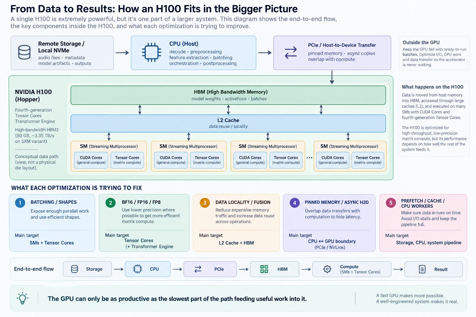
One of the easiest mistakes to make with an H100 is assuming that owning an extremely fast GPU means you have an extremely fast AI system. I ran into this while working on a production audio-analysis workload that processed thousands of recordings every day. Each recording passed through signal-processing code, CPU preprocessing, several AI models, post-processing, and persistence. The workload ran as a scheduled batch job, primarily around a single H100, and once it became part of a daily production process, its total completion time mattered much more than the speed of any individual model.

This was a different system from the speaker-based fraud-detection pipeline I have written about elsewhere. I will leave the business logic out of this article, but the engineering problem is more interesting anyway: given a heterogeneous pipeline, several models, variable-length inputs, network and storage I/O, CPU-bound work, and one very capable accelerator, how do you maximize the amount of useful work that gets completed before the next daily run?

After profiling and restructuring the system, we reduced the end-to-end runtime by roughly 75%. The H100 itself did not become faster. The majority of the work was about removing the reasons the rest of the system prevented it from being useful.

The metric was the job, not the GPU

My first principle became simple: optimize the metric the business is actually waiting for. In this case that was the completion time of the entire daily job. GPU utilization, VRAM allocation, inference latency and CPU utilization were diagnostic signals, but none of them was the objective on its own. For an offline workload, the useful metric was essentially completed recordings per unit of wall-clock time, together with the guarantee that the complete batch could finish comfortably inside its processing window.

That distinction matters because a GPU can look busy without producing good system throughput, and it can occasionally look underutilized while the system is behaving perfectly reasonably. Filling 80 GB of VRAM is not a measure of success either. Neither is reaching an aesthetically pleasing number in nvidia-smi. What matters is whether another change causes more real production work to finish in less time without damaging correctness or reliability.

The first thing I therefore wanted was an end-to-end performance decomposition. At a simplified level, the path looked like this:

storage / network
       ↓
audio decode
       ↓
signal processing
       ↓
CPU preprocessing
       ↓
host → device transfer
       ↓
GPU model A
       ↓
GPU model B
       ↓
post-processing
       ↓
persistence

I instrumented the boundaries rather than treating inference as a black box. For every meaningful stage, the useful numbers were total time, time per input, throughput, queue wait, batch size and the distribution of input sizes. At the infrastructure level I also cared about CPU saturation, I/O throughput, GPU activity, VRAM, host memory and the behavior of the queues connecting stages. Once those numbers were visible, several assumptions about where time was being lost became much easier to challenge.

This is also where Amdahl's law becomes very practical. Making a model twice as fast cannot halve the runtime of a pipeline if that model represents only a small part of the critical path. Conversely, removing a seemingly boring I/O stall that repeatedly leaves an H100 with nothing to do can have a surprisingly large effect on total runtime.

The first enemy was serialization

A perfectly reasonable first implementation of an AI pipeline often looks like this:

for item in items:
    audio = load(item)
    features = preprocess(audio)
    output = model(features)
    result = postprocess(output)
    save(result)

The problem is that this code serializes resources that do not need to be serialized. While the system waits for storage, the CPU and GPU may be idle. While preprocessing is happening, the H100 may have nothing to execute. While a result is being persisted, the next batch may not yet be preparing. A very expensive accelerator can end up spending a meaningful portion of the job waiting for Python, CPUs, disks or the network.

The better mental model was a pipeline of independent producers and consumers. While the H100 processes batch N, CPU workers can prepare batch N+1, I/O workers can prefetch future inputs, and another stage can persist the results of batch N-1. This does not mean maximizing parallelism indiscriminately. It means overlapping work that uses different resources and has no dependency requiring it to be serialized.

Conceptually, I wanted the machine to behave more like this:

The interesting unit of optimization stopped being a recording and became the flow of work through the complete system.

I/O deserves the same attention as inference

Storage is easy to ignore because it feels like infrastructure rather than AI, but a GPU that waits for data is an I/O problem regardless of how impressive the model is. In a production batch pipeline I want to know whether input data is local or remote, whether I am performing many small network reads, whether the same objects are repeatedly downloaded, whether audio decoding keeps up with inference, whether outputs are written synchronously in the hot path, and whether databases are receiving one request per recording when they could receive a batch.

The solution depends on where the measurements point. Network-bound inputs can be prefetched with a bounded number of I/O workers. Frequently reused artifacts can be staged locally. When remote object storage becomes part of the critical path, a local NVMe staging area can be much more valuable than another inference optimization. Metadata should be fetched efficiently rather than through thousands of unnecessary round trips. Writes that do not need to block inference can be moved behind a queue. Database inserts, vector operations and other persistence work should generally be batched when the backend supports it.

The important part is to separate I/O concurrency from compute concurrency. Threads are often useful for operations that spend their time waiting on a network or storage service. Increasing GPU workers is a completely different decision. I want separate limits for each resource because they have different saturation points.

I also try to reduce data movement itself. If a pipeline repeatedly copies large arrays between representations, serializes and deserializes the same intermediate data, or moves tensors between CPU and GPU more times than necessary, that overhead eventually becomes visible once inference is fast enough. Data layout and movement are part of performance engineering.

Batching is where the H100 starts to make sense

An H100 contains far more parallel compute than a single short audio sample can use effectively, which makes batching one of the most important throughput controls. Instead of submitting one small piece of work and waiting for it to complete, the goal is to give the accelerator enough independent work to exploit the hardware it contains.

But “increase the batch size” is incomplete advice. The useful question is where the throughput curve stops improving relative to the additional memory and operational risk. I prefer to sweep realistic batch sizes and measure completed work per second rather than decide that the largest batch fitting in VRAM must be the best one.

Audio adds another problem because inputs are variable in length. If a four-second recording shares a padded batch with a sixty-second recording, a large amount of compute can be spent processing padding rather than signal. Bucketing inputs by approximate duration makes batches more homogeneous:

Arbitrary batching:
 
4s    8s    13s                         61s
|----|-----|--------|--------------------|
 
Duration-aware batching:
 
Batch A:  4s   5s   7s   8s
Batch B: 48s  52s  57s  61s

This improves the useful work done inside a batch and makes memory consumption more predictable. It also highlights why synthetic benchmarks can mislead. A benchmark containing uniformly short recordings may tell you almost nothing about the batch-size behavior of a production day containing a long-tailed duration distribution.

For offline jobs I also care about the tail of that distribution. If all the long recordings are left until the end, most workers can become idle while a handful of stragglers determine when the entire job finishes. Duration-aware scheduling can therefore improve both batch efficiency and end-of-job behavior. Sometimes starting expensive items earlier is useful simply because the completion time of the slowest remaining work defines the batch deadline.

Concurrency should be controlled, not maximized

Once people see idle periods, the natural reaction is often to add workers. That works until it does not. If four CPU workers already prepare data faster than the GPU can consume it, increasing that number to thirty-two will not make the H100 faster. It can instead increase memory use, filesystem contention, scheduler overhead and competition between numerical libraries that already create their own threads.

I prefer thinking in terms of independently constrained concurrency domains:

                 ┌─────────────────┐
storage/network →│   I/O workers   │
                 └────────┬────────┘
                          │
                    bounded queue
                          │
                 ┌────────▼────────┐
                 │   CPU workers   │
                 └────────┬────────┘
                          │
                    bounded queue
                          │
                 ┌────────▼────────┐
                 │ batching / H100 │
                 └────────┬────────┘
                          │
                    bounded queue
                          │
                 ┌────────▼────────┐
                 │ postprocess /   │
                 │ persistence     │
                 └─────────────────┘

Bounded queues are important here because they provide backpressure. If the GPU is slower than the producers feeding it, upstream stages eventually block instead of allocating memory indefinitely. If the GPU queue repeatedly becomes empty, I immediately know that something upstream is failing to feed it quickly enough. Queue depth becomes an extremely useful performance signal.

This is also why the right number of workers is usually found experimentally. I increase concurrency while measuring throughput, queue behavior, CPU saturation, memory usage and I/O performance. Once throughput stops improving, additional workers are usually only creating more contention. The objective is a balanced pipeline, not the largest thread pool I can configure.

Several models turn the problem into scheduling

The pipeline became more interesting because it used several AI models rather than one homogeneous inference step. Multi-model workloads introduce a scheduling question that single-model benchmarks largely avoid: what should be resident on the H100, what should run when, and what should the unit of scheduling be?

There are two simplified extremes:

Item-oriented:

item 1 → model A → model B → model C
item 2 → model A → model B → model C
item 3 → model A → model B → model C

and:

Stage-oriented:

items 1...N → model A
                   ↓
items 1...N → model B
                   ↓
items 1...N → model C

The first can be attractive for latency-sensitive systems because an individual item reaches the end quickly. The second can be attractive for offline workloads because it creates much better opportunities for batching and amortizes setup and model-switching costs over more work. Stage-oriented execution also has costs: intermediate artifacts need to be managed, failures need to be resumable between stages, and total orchestration becomes more sophisticated.

The key is that an offline cron job and an online request-serving API should not automatically have the same execution architecture. One is usually dominated by throughput and deadline constraints; the other often has strict per-request latency requirements. Optimizing them with the same strategy can be a mistake.

Model residency is part of the same problem. Loading a model, moving its weights to the device, initializing runtime state and warming up kernels are all costs. Repeating those operations for small pieces of work destroys throughput. At the other extreme, keeping every model resident merely because 80 GB of HBM makes it possible can create memory pressure without improving execution.

I want to know which models are used frequently enough to stay resident, whether grouping work by model avoids unnecessary swaps, whether multiple models actually benefit from concurrent execution, and whether they compete for the same compute or memory bandwidth when run together. Two models fitting in VRAM says nothing about whether executing them concurrently is faster.

For some underfilled workloads, independent CUDA streams or process-level concurrency can improve overlap. For others, they simply create contention. That is something to benchmark on the actual model mix rather than assume.

Host-to-device movement can become the next bottleneck

Once the larger architectural issues are fixed, smaller details become worth investigating. The H100 needs its inputs in device memory, and repeatedly waiting for synchronous host-to-device transfers can create bubbles between batches.

When transfers show up on the critical path, pinned host memory and asynchronous transfers can allow copies to overlap with GPU execution. A common pattern is conceptually:

GPU computes batch N
 
while:
 
CPU prepares batch N+1
and
batch N+1 begins transferring to the device

In frameworks such as PyTorch this can involve pinned DataLoader memory, non-blocking transfers and carefully used CUDA streams. The qualification matters: these mechanisms do not automatically make a pipeline faster. They are useful when profiling shows transfer or preparation gaps that can actually be overlapped. Adding asynchronous complexity to a pipeline whose bottleneck is somewhere else only makes the code harder to operate.

I also try to avoid unnecessary device round trips. If the output of one GPU stage can feed another stage directly, sending it back to CPU only to upload it again later may be wasteful. Whether it is worth keeping intermediate tensors on device depends on memory pressure, model scheduling and whether CPU-side post-processing is required, but it is a decision worth making intentionally.

Use the H100's numerical capabilities when the model allows it

After the pipeline is feeding the accelerator properly, model-runtime optimization becomes much more meaningful. An H100 is designed to perform low-precision tensor operations extremely efficiently, so running every compatible model in FP32 by default can leave a large amount of performance unused.

For inference workloads I generally evaluate BF16 or FP16 where the model and operators support them and verify that the change does not create an unacceptable quality regression. BF16 is particularly attractive for many modern models because of its wider exponent range. FP8 can provide another level of throughput on Hopper hardware for compatible workloads, but I treat it as an optimization that requires explicit validation rather than something to enable because the hardware supports it.

The same principle applies to inference-specific execution. Models should be in evaluation mode and run without autograd when gradients are unnecessary. In PyTorch, torch.inference_mode() removes work that an inference pipeline does not need. Stable hot paths can also be candidates for compilation or optimized runtimes such as torch.compile, ONNX Runtime or TensorRT, depending on the model and deployment constraints.

These optimizations can be extremely valuable, but I deliberately put them after the system-level discussion because it is easy to spend days shaving milliseconds from kernels while the accelerator waits hundreds of milliseconds for the next batch. Kernel optimization has much higher leverage after the pipeline stops starving the kernel.

Stable shapes can unlock another layer of optimization

Dynamic production inputs are convenient for application developers but often less friendly to optimized execution. Highly variable tensor shapes can cause additional allocations, prevent some compilation optimizations and reduce opportunities for graph reuse.

Duration bucketing helps here too because it reduces shape variability within batches. When a model is repeatedly invoked with a small set of predictable shapes, it becomes easier for compilers and optimized runtimes to produce efficient execution plans. In sufficiently stable workloads, CUDA Graphs can reduce repeated launch overhead by capturing and replaying an execution sequence, although the constraints around memory addresses and shapes mean that this technique is not appropriate for every pipeline.

The general lesson is that regular workloads are easier to optimize than chaotic ones. Sometimes performance comes from converting a highly dynamic stream of individual inputs into a small number of well-defined execution classes.

Memory should be managed for throughput, not aesthetics

The H100 has enormous memory capacity, but VRAM is still a resource that needs a strategy. Maximum allocation is not maximum efficiency. I want enough memory to support useful batches and resident models while retaining headroom for production variance, runtime workspaces and unusual inputs.

This is especially important for variable-length workloads. A configuration that consumes 79 GB on a carefully selected benchmark can become an intermittent OOM failure when a real batch contains several unusually large inputs. An extra few percent of benchmark throughput is rarely worth turning a daily production job into something that occasionally dies at 3 a.m.

Repeated allocation and deallocation can also matter in long-lived inference processes. Where practical, stable tensor shapes and buffer reuse reduce allocator churn. I avoid treating calls such as clearing a framework cache after every batch as a performance strategy; frequent forced cache eviction can simply create additional allocations later. Memory behavior should be measured over the complete steady-state workload.

The CPU is part of the AI system

A powerful GPU makes weak CPU pipelines easier to expose. Audio decoding, resampling, feature extraction, signal processing, data transformations and serialization can consume enough CPU time to starve the accelerator.

The first optimization is to determine which work is actually CPU-bound. I/O-bound operations often benefit from threads, while CPU-heavy Python work may need processes or native/vectorized implementations. Numerical libraries can themselves use multiple threads, which means multiplying process count by internal thread count can accidentally oversubscribe the machine. A pipeline with eight workers each attempting to use eight CPU threads can behave substantially worse than a deliberately constrained configuration.

I also look for work that can be vectorized or moved out of Python loops, repeated conversions between libraries, unnecessary copies, and transformations that can be computed once and reused. As the GPU becomes faster, these details represent a larger fraction of the critical path.

The useful question is whether the GPU input queue ever drains because the CPU cannot produce the next batch. When that happens, the CPU has become a GPU-performance problem.

Caching can outperform optimization

The fastest version of an expensive model invocation is still slower than not invoking the model.

Batch pipelines create many opportunities to exploit that fact. If a deterministic preprocessing stage has already completed for an unchanged input, its output may be reusable. If a recording has already been transferred from remote storage into the processing environment, it should not necessarily be transferred again. If a model stage completed successfully before a downstream failure, rerunning that stage might be unnecessary.

This requires designing artifacts and identities deliberately. Inputs can have stable identifiers or content hashes. Stage outputs can be associated with the model and preprocessing version that produced them. A manifest can record which work has completed. Changing a model should invalidate the outputs that depend on that model without forcing unrelated stages to run again.

The cache key matters as much as the cache. Conceptually, I want something closer to:

artifact =
    f(
        input identity,
        preprocessing version,
        model version,
        relevant configuration
    )

rather than simply "this filename exists, therefore reuse it."

That makes caching reproducible instead of accidental.

Caching also changes recovery behavior dramatically. Suppose a job contains 10,000 recordings and fails after 8,700 have successfully completed an expensive stage. A naïve restart performs 10,000 expensive operations again. A resumable pipeline performs the remaining 1,300. No tensor-core optimization is going to beat eliminating 8,700 unnecessary executions.

Idempotency is a performance feature

I used to think about idempotency mainly as a reliability property. In large AI batch jobs it is also a resource-efficiency property.

Scheduled jobs will eventually encounter failures. A network request times out, an input is malformed, an external service becomes unavailable, a process is killed, or a deployment happens during execution. The pipeline should know what is complete, what failed, and what remains. Retrying one failed item should not require replaying an entire day's GPU work.

This changes how I structure long jobs. Stages should checkpoint meaningful progress. Writes should be safe to retry. Individual failures should be isolated rather than crash unrelated work where possible. Failed items can move to a retry or dead-letter path while the rest of the workload continues. Temporary files should have clear ownership and cleanup behavior. A restarted cron job should converge toward the correct final state instead of duplicating outputs.

Reliability and performance meet here because every unnecessary replay consumes the same CPU, storage and GPU capacity that the optimization work was trying to preserve.

Backpressure is better than hidden overload

A production batch system can appear fast temporarily simply because one stage is producing work much faster than another can consume it. If queues are unbounded, the imbalance gets hidden in RAM until the process slows down, swaps, runs out of memory, or fails.

Bounded queues force the system to reveal its true sustainable rate. When a downstream stage saturates, producers wait. This is useful. It prevents load from being transformed into memory pressure and gives queue depth a clear meaning.

A good performance dashboard for a pipeline therefore includes more than GPU metrics. I want to see per-stage throughput, queue depth over time, queue wait time, batch fill rate, input-size distributions, retry counts and failure rates. If the queue before the GPU is always full, the accelerator or its execution strategy may be the limiting stage. If it repeatedly reaches zero, the accelerator is being starved. If the queue after the GPU grows continuously, the bottleneck has moved downstream.

Performance engineering becomes much easier when the architecture exposes its bottlenecks rather than masking them.

Warm-up and steady state need to be separated

Another source of misleading measurements is benchmarking cold execution together with steady-state execution. The first batch can include model loading, CUDA context creation, kernel initialization, compilation, memory allocation and filesystem cache misses that do not represent the remaining thousands of inputs.

For capacity planning I care about both numbers, but they answer different questions. Cold-start cost matters for short-lived jobs and model-switching strategies. Steady-state throughput determines how quickly a large daily workload moves once the system is running.

This is especially important when evaluating model residency. If a model takes meaningful time to initialize but processes thousands of items afterward, that cost is amortized easily. If the pipeline constantly loads and unloads that model for tiny groups of inputs, the same initialization cost can become significant.

A benchmark should therefore use representative production inputs, include an explicit warm-up phase where appropriate, and measure long enough for the system to reach stable behavior.

Optimize the critical path, then profile again

Performance work is iterative because fixing one bottleneck exposes the next one. Faster preprocessing can make inference dominant. Better batching can make storage visible. Faster GPU execution can expose a post-processing step that previously looked irrelevant. Adding a cache can reduce model work enough that network latency suddenly becomes a larger fraction of the job.

My optimization loop is therefore deliberately boring:

measure
   ↓
identify the current limiting stage
   ↓
form a hypothesis
   ↓
change one thing
   ↓
measure end-to-end throughput again
   ↓
keep or revert
   ↓
repeat

This is also why I like having a fixed representative benchmark set. Performance changes should be repeatable, and they should be evaluated against the same workload shape. Otherwise it becomes easy to attribute a fast day to an optimization when the batch simply contained shorter or easier inputs.

I also avoid judging an optimization only by its local metric. If preprocessing becomes 50% faster but the end-to-end job improves by 0.5%, that is useful information. It means preprocessing is probably no longer where engineering time has the most leverage.

Observability is part of performance engineering

Once a pipeline is optimized, it needs to remain optimized. Workloads change, input distributions drift, model versions change, libraries are upgraded and storage behavior changes. A configuration that worked well three months ago may slowly become suboptimal without anybody touching the scheduling code.

For each production run I therefore want enough information to reconstruct its performance: total runtime, number and duration distribution of inputs, per-stage timings, effective batch sizes, queue behavior, retries, failures, CPU consumption, GPU memory usage and relevant model/configuration versions. Aggregate averages are useful, but p95 and tail behavior often explain why one daily run took dramatically longer than another.

Monitoring this over time also turns optimization into capacity planning. If the number of daily inputs doubles, I can estimate whether the existing H100 still has headroom, whether a specific CPU or I/O stage will become the first bottleneck, or whether additional accelerator capacity will eventually be justified.

That is a much better position to be in than discovering the limit when the cron job stops finishing before the next one starts.

The 75% was the result of the system, not one trick

Across the accumulated changes, the end-to-end runtime fell by roughly 75%. There was no single magical optimization responsible for the result. It came from treating the entire execution path as one system: measuring first, increasing useful batch work, handling variable-length inputs intelligently, overlapping independent CPU, I/O and GPU stages, avoiding unnecessary model setup, controlling concurrency, reducing data movement, reusing completed work, making retries incremental, and continuously moving attention to whichever stage became the new bottleneck.

Only after those architectural issues were under control did lower-level inference optimizations become especially valuable. Precision choices, optimized runtimes, asynchronous transfers and similar techniques matter, sometimes substantially, but their impact is constrained by everything surrounding the model.

The H100 never became faster. We simply stopped making it wait so much, stopped giving it inefficient work, and stopped asking it to repeat work that had already been done.

That distinction is the main thing I took from the project.

How I now approach an expensive GPU that looks too slow

When I encounter a slow production AI workload today, I do not begin by asking how to increase GPU utilization. I first define the unit of useful work and measure its end-to-end rate. Then I trace the critical path from storage to output and ask what prevents the next useful batch from reaching the accelerator.

I look at the data path: are we waiting on remote storage, doing redundant reads, writing synchronously, or making thousands of small database requests? I look at CPU preparation: can preprocessing keep up, is it oversubscribed, and are we copying or transforming data unnecessarily? I look at batching: are batches large enough, are variable-length inputs creating padding waste, and where does the throughput curve flatten? I look at model scheduling: which models should remain resident, which work should be grouped by model, and is concurrent execution actually helping? I look at the host-to-device path and whether copies can overlap with compute. Then I look inside inference itself: numerical precision, runtime choice, compilation, kernel behavior and stable shapes.

Finally, I look for work that should disappear entirely through caching, incremental processing, checkpointing and idempotent recovery. In many production systems that last category produces some of the cheapest performance wins available.

An H100 gives a system an enormous amount of computational capacity. Making use of that capacity is an ML systems problem. The model matters, but so do the queues before it, the storage behind it, the CPU feeding it, the way inputs are shaped, the way several models share the device, and what the application decides it does not need to calculate twice.

That is the difference between having an H100 and actually getting H100-class throughput out of a production workload.